
Figure 0. The Mandelbrot set.
Home > Essays > An explanation of the Mandelbrot set for artists (continued)
In the previous page, you read about iteration and complex numbers, and how these two concepts come together in the Mandelbrot set. The Mandelbrot set is in turn of great importance to a type of Julia sets, which is where we now pick things up.
 Gaston Julia as a young man, playing the violin, before the horrific World War I incident in which he lost his nose.
The French mathematician Gaston Julia studied iteration and complex numbers long before computers made it practical to draw diagrams of the sets that are now called Julia sets in his honor.
The basic principle of a Julia set is the same as the Mandelbrot set: iterate the function across points of the complex plane and some points will escape to infinity and some points will attain stable orbits.
The functions we're concerned with here are quadratic functions. A quadratic function takes in a number, squares it, and maybe also adds or subtracts a number. Algebraically, we can write f(z) = z2 + c; we understand that c doesn't have to be a positive real number, it can just as easily be 0, a negative real number, an imaginary number or a complex number.
The expression f(z) = z2 + c looks a lot like the expression for the function we iterated to get the Mandelbrot set, but there is one important though subtle difference here. I will try to explain it as clearly and as simply as I can.
With both the Mandelbrot set and Julia sets, we look (or we have the computer look) at points in an area of the complex plane one by one. We can express a point as x + yi.
For the Mandelbrot set, we set c = x + yi and the first value of z to either z = 0 or z = c. Then, after making the determination of escape or stable orbit, we move on to the next point, which means a new x + yi and consequently a new c = x + yi.
With the Julia set of a quadratic function, we first select a value of c before we do anything else. For the first point x + yi that we look at, we set z = x + yi, but we don't change c. We make the determination of escape or stable orbit and move on to the next point, a new z = x + yi, using the same value of c for all the points.
What this means in practical terms to you as a computer user is that before your program, be it FractInt or whatever, can draw you a Julia set of a quadratic function, you have to specify the value of c to be used. (Since I'll only be going over Julia sets of quadratic functions on this page, I will just write "Julia sets" for the rest of this page).
| n | zn, z0 = 1 | zn, z0 = i |
|---|---|---|
| 1 | 1.25000000 | −0.75000000 |
| 2 | 1.81250000 | 0.81250000 |
| 3 | 3.53515625 | 0.91015625 |
| 4 | 12.74732971 | 1.07838440 |
| 5 | 162.74441478 | 1.41291291 |
| 6 | 26485.99454347 | 2.24632290 |
| 7 | *** | 5.29596657 |
| 8 | *** | 28.29726190 |
| 9 | *** | 800.98503076 |
| 10 | *** | 641577.26950257 |
Let's look now at a concrete example, c = 1/4 = 0.25. The first point we will look at is z = 0. As it turns out, we already went over this in the previous page (see Table 1 there). This iterated function does not settle on a specific value, but it certainly does not escape to infinity, instead slowly getting progressively closer and closer to 1/2.
With the same c = 1/4, let's now look at z = 1. The escape is fairly fast, giving us 5/4 = 1.25, 29/16 = 1.8125, 905/256 = 3.53515625, 835409/65536 = 12.7473297119140625, etc. It should be obvious that z = −1 gives the same escape (remember, the square of a negative real number is a positive real number).
One more z before we hand it over to the computer, z = 1 + i. The escape is much faster, though to a directionless infinity rather than positive real infinity.: 1/4 + 2i = 0.25 + 2i, −59/16 + i = 3.6875 + i, 3289/256 − 59i/8 = 12.84765625 − 7.375i, etc.
Now let's turn it over to the computer.
Kind of reminds me of broccoli, and just about as uninteresting. But it's still more interesting than the Julia set with c = 0 (which just produces a plain old circle).
We get a much more interesting Julia set if we move c away from 0 and towards −1, such as c = −3/4 = −0.75, to get a Julia set that is sometimes called "the San Marco dragon."
 The San Marco dragon fractal over a photo of the Basilica di San Marco in Venice, Italy. If you filled the piazza with water up to a certain point, the resemblance would be much more striking.
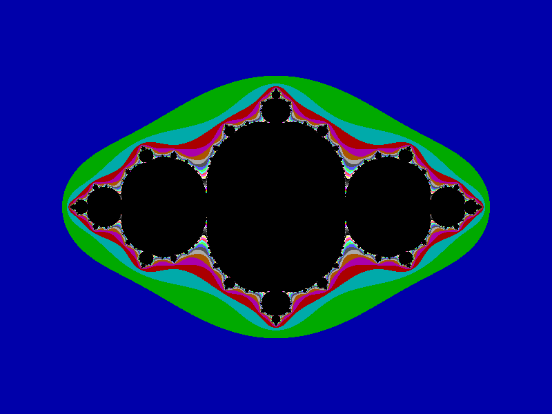
Kinda reminds you of the Mandelbrot set, doesn't it? So that's two examples in a row of Julia sets with c purely real. Here's one with c imaginary, namely, c = i.
This Julia set is sometimes called a "dendrite," because it kind of looks like a short branched extension of a nerve cell. In this picture you can barely see the stable orbit points at all, but I assure you, they're there, and they're all pathwise connected.
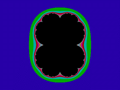
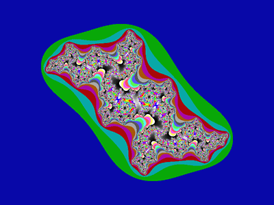
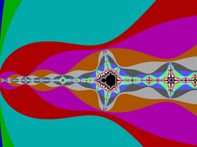
Now let's try some values of c having both a real part and an imaginary part, such as c = −0.51 + 0.56i.
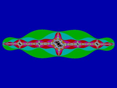
The sign of the imaginary part of c does not seem that important, as changing it just flips the Julia set along the imaginary axis:
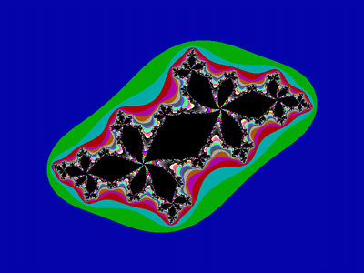
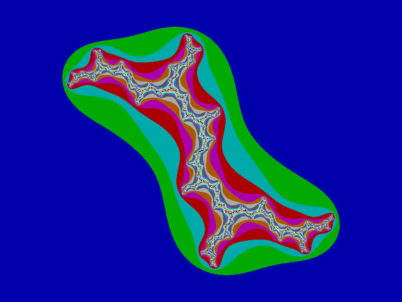
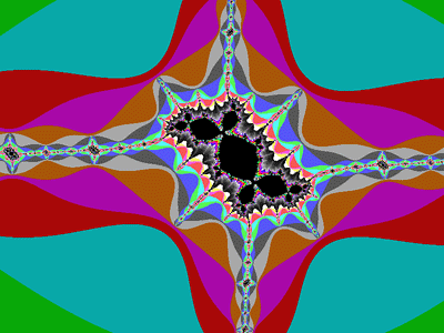
These last two Julia sets are very similar to a Julia set sometimes called "the Douady rabbit" (named after the relatively recently deceased French mathematician Adrien Douady), with c ≈ −0.125 + 0.741i (don't get too hung up on being precise with this number; I will explain the allowable variance very soon).
A couple of observations based on the examples so far. First, like the Mandelbrot set, most Julia sets exhibit self-similarity, and it can be quite interesting to zoom in and look at the boundary between the stable orbit points and the escaping points.
Second, Julia sets have symmetry along the real axis, and if Im(c) = 0 (meaning that c is purely real), the Julia set also has symmetry along the imaginary axis.
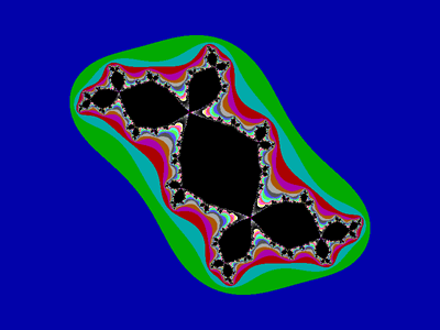
The stable orbit points of the Douady rabbit are all pathwise connected, though the connections are very narrow in certain spots. With a slight adjustment of c, we can get a variation of the Douady rabbit in which the stable orbit points are disconnected:
How can we tell if the stable orbit points of a Julia set are pathwise connected or disconnected without having to draw the set?
The answer is in the Mandelbrot set. If c is a stable orbit point in the Mandelbrot set, then the corresponding Julia set has its stable orbit points all pathwise connected.
But if c is not a stable orbit point in the Mandelbrot set, then the corresponding Julia set has its stable orbit points disconnected, or it has no stable orbit points at all.
There is also a correlation between the shape of a Julia set and the position of c in the Mandelbrot set. Although c = 0 is not the central point of the Mandelbrot set, it is the center of the complex plane, and its corresponding Julia set, the plain circle mentioned earlier, could be considered the basic Julia set.
As we move c a little bit away from 0, keeping it within the "main part" of the shape (the biggest part, sometimes called a cardioid) the corresponding Julia set looks a pinched circle.
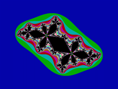
Moving c "upward" or "downward" into the attached smaller shapes of the Mandelbrot set pinches the circle of the corresponding Julia set in such a way as to look more like a boldface letter Z. Moving c towards the thin rays gives a Julia set that itself looks like a thin ray.
Hence this chart:
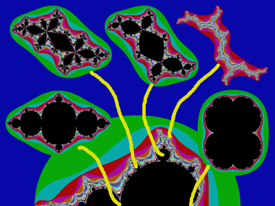
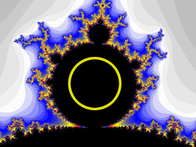
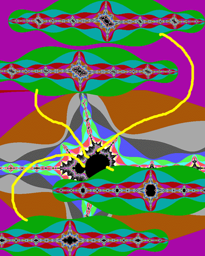
From this chart, it is reasonable to think that the Douady rabbit doesn't have to have c = −0.125 + 0.741i precisely. I find it easier to remember it as c = −1/8 + 3i/4 = −0.125 + 0.75i; you can move c as much as 1/10 in any direction and still get the Douady rabbit. In the following Mandelbrot set zoom, I have drawn a yellow circle around an area. I think that if you choose any c within that area, the corresponding Julia set will look quite well enough like the Douady rabbit.
A nice feature of WinFract (and I'm guessing FractInt has this feature as well) is Mandelbrot/Julia toggling. If you right-click on a point c on or off the Mandelbrot set diagram displayed in that program, the program will draw the corresponding Julia set for c. And if you right-click again, the program takes you back to the Mandelbrot set.
Obviously you have to be precise on where you click on the Mandelbrot set, but I'm not sure if you also have to precise on where you click on the Julia set. I've occasionally confused myself after a toggle.
Do you remember this zoom of the Mandelbrot set from the previous page?
If you have WinFract on the Mandelbrot set, I want you to zoom in on WinFract and right-click on the area of the "little Mandelbrot" that's shaped like the area in which I put the yellow circle in Figure 17.
What's this? Is there a little Douady rabbit in there? Zoom in:
Yes, there is! And what's more, there are even smaller Douady rabbits that are all connected together by thin filaments. I'm giving you the coordinates −1.7575755 + 0.0057633i. It is important to be precise with this number, because, although as with c = −0.125 + 0.75i, there is room for variance, for this point the room for variance to get a little Douady rabbit is quite small.
We can go one step further and create a diagram for this little Mandelbrot that is very similar to what Figure 16 is for the whole shape.
The absence of a small dendrite from Figure 19 does not necessarily mean that it's not there to be found, it just means that I wasn't able to find it. Even if it does not actually exist, it does not detract from my amazement at finding these "little" Julia sets.
You can also get little Douady rabbits that are not neatly aligned on the real number axis by Mandelbrot/Julia toggling at the appropriate spots on "little Mandelbrots" that are not themselves on the real number line, like the one shown in Figure 8b.
And so we see that the self-similarity of the Mandelbrot set also extends to its correspondences to Julia sets. After twenty years of knowing about the Mandelbrot set and its relation to Julia sets, I can still find things in it that surprise me.
WinFract saves images in the Graphic Interchange Format (GIF) with an uppercase extension, and I'm guessing this is also the case with FractInt. This is probably a non-issue unless you want to upload the output of these programs to a website and the server is case-sensitive.

In the case of this website, changing the filenames to lowercase with Windows was easy, but in some instances I actually used the DOS command line to change the extensions to lowercase (that was a blast from the past).
File size is perhaps more important than the filenames and extensions being in upper or lowercase. I did not change WinFract's default for image size, so it gave me GIF files of 800 by 600 pixels. I thought if I scaled these images down to 400 by 300, the files would be smaller.
Well, much to my surprise, some of the image files took up more kilobytes for fewer pixels. It therefore made more sense to upload the smaller files with more pixels instead and scale them down to the dimensions I wanted by using HTML (I guess I should have used CSS to accomplish that, but I can always take care of that later). You can tell which ones these are by searching the source of this page for width="400" height="300".
Also, be mindful of the indexed color mode. You might change the mode to RGB or CMYK, make some alterations to the image, then find that when you switch it back to indexed color you lose the color savings of indexed color.
Having fewer colors in the palette does not result in much file size savings if the fractal shape is so elaborate that the compression algorithm can't do much with it. If you're very interested in the boundary of the stable orbit points and not at all interested in the distinction between quickly and slowly escaping points, then you might be able to use Photoshop's Threshold command to get rid of all that extra stuff (that's what I did for Figure 6).
But what is perhaps the most important practical consideration here is that WinFract does not save coordinate data with the image, which means that if you zoom in a lot and don't write down the coordinates, you might be unable to find your way back later. Don't learn it the hard way: write down coordinates and attach them to the images somehow.
I don't know if ChaosPro saves coordinate data or not, but then again, currently there's much about ChaosPro that I don't really know.
If I simply took the output of WinFract and claimed it as my own art, that would be wrong, in my opinion. Although there are certain decisions to be made as the human operator of a fractal program (like the color maps, for one), the way I see it, these are things that have always existed and will always exist, regardless of whether or not there are humans to appreciate them.
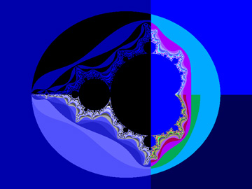
When you modify the output of a fractal program to include other imagery, that's when you start getting into actual art. Although I hesitate to claim the overlaying of the San Marco dragon (Figure 11) over the photo of the Basilica as artwork, it might point in an interesting direction artistically, one that I might explore further.
The default colors in FractInt may be too garish for your taste, and the ones in ChaosPro too muted. Rather than learn how to change the colors in those programs, it might be much more effective to make the changes in Photoshop or Photoshop Elements.
All the means for adjusting colors that are available for photos are also available for images from fractal programs. Just make sure to change the color mode from indexed to RGB, CMYK or grayscale.
I know quite a few painters with a phenomenal skill for incorporating amazing levels of detail into their paintings. To them I am obligated to give a reminder that whatever diagram you see on a screen or in a book is only a finite approximation.
Instead of trying to reproduce all the detail you see in the fractal program, you should use the power of suggestion to imply the infinite self-similarity, rather than trying to be precise with every little dot or filament.
And I certainly recommend against trying to paint the escaping points as you see them in the fractal program. As a painter who now has some understanding of the mathematical underpinnings of these diagrams, you ought to feel free to interpret the escaping points in whatever way you want.
Although it would not seem to be of direct relevance to fractals, Neil Sloane's On-Line Encyclopedia of Integer Sequences has been a valuable resource in the writing of this page. For example, Sloane's A072191 was just one of many sequence entries I looked up as I wrote this page.